Chapter 2 From Dirichlet Distribution to Dirichlet Process
2.1 Dirichlet Distribution
Dirichlet Distribution is a distribution over the relative values of \(K\) components, and the sum of them must be restricted to be \(1\). The parameter of the distribution is a \(K\)-dimensional vector \(\alpha = (\alpha_1, \alpha_2, \alpha_3,...,\alpha_K)\), where \(\alpha_k > 0\). The probability density function of Dirichlet distribution is
\[\pi = (\pi_1, \pi_2, \pi_3, \dots ,\pi_K)\sim Dir(\alpha_1, \alpha_2, \alpha_3,\dots,\alpha_K) = \frac{\displaystyle\prod_{k = 1}^{K} \Gamma(\alpha_k)}{\Gamma(\displaystyle\sum_{k = 1}^{K}\alpha_k)}\displaystyle\prod_{k = 1}^{K}\pi_k^{\alpha_k - 1}\]
where \(\Gamma(\cdot)\) denotes the Gamma function.
The expected value of Dirichlet distribution is
\[E[\pi] = \frac{\alpha}{\displaystyle\sum_{k = 1}^{K}\alpha_k},\text{ where } \pi \text{ and } \alpha \text{ are vectors.}\] In the density plot below, we can observed that the position of the expected value has the highest density.
Figure 2.1 visualizes the Dirichlet distribution density plot in \(\mathbb{R^3}\) under different parameters. In these \(4\) density plots, red areas have a high density, while blue area have a low density. In the top-left graph, \(\alpha = [1,1,1]\), the Dirichlet distribution is equivalent to a uniform distribution. In the top-right graph, \(\alpha = [c,c,c], 0<c<1, c = 0.1\), the distribution is symmetric and has higher density on the edges. In the bottom-left graph, \(\alpha = [c,c,c], c>1, c = 10\), the distribution is symmetric and has the highest density at \([\frac{1}{3}, \frac{1}{3}, \frac{1}{3}]\). In the bottom-right graph, \(\alpha\) is not in the form of \([c,c,c]\) so it is not symmetric. It has the highest density at \([\frac{1}{11}, \frac{5}{22}, \frac{15}{22}]\). Figure 2.2 shows the distribution of samples drawn from these \(4\) Dirichlet distributions. The method of generating samples from a Dirichlet distribution will be showed later in this chapter.
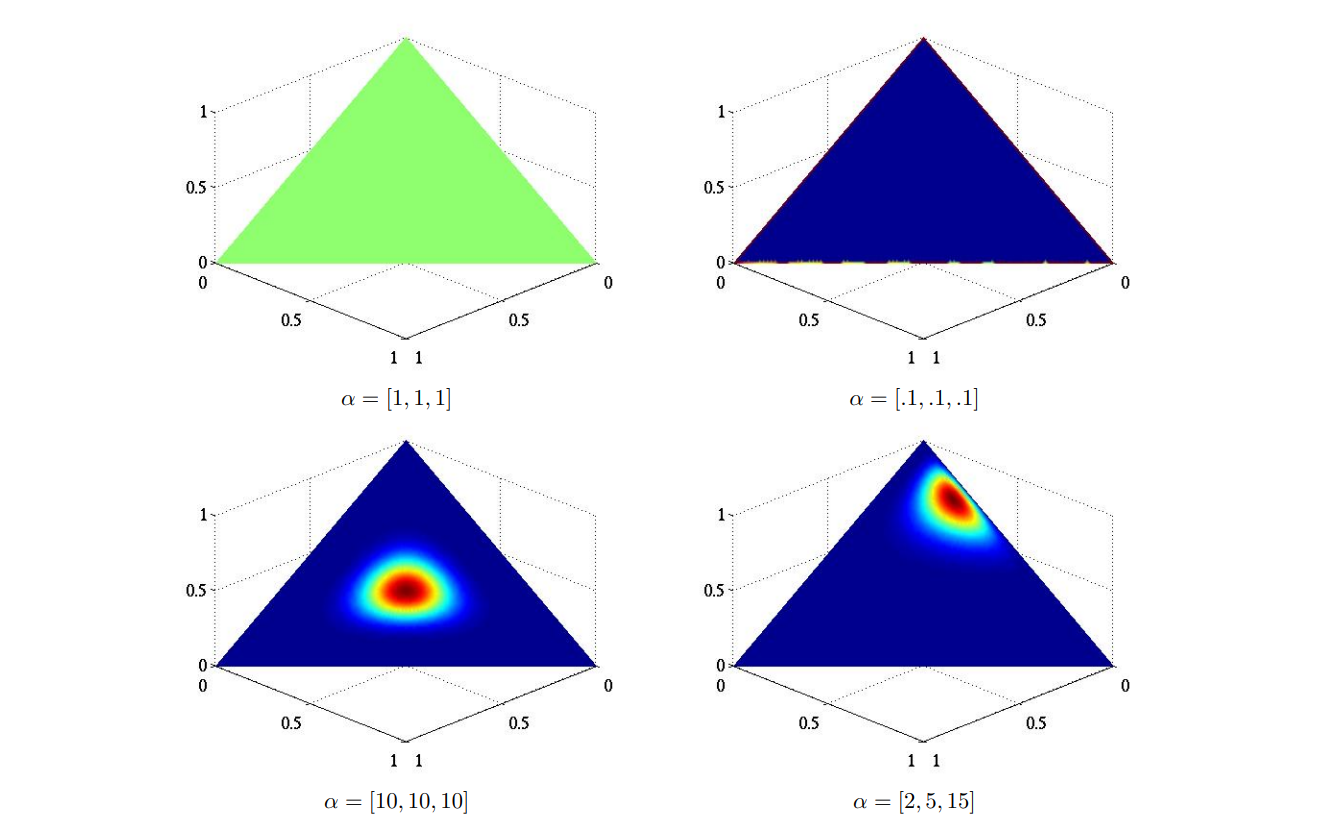
Figure 2.1: Visualization of Dirichlet distribution density (Frigyik, Kapila and Gupta, 2010)
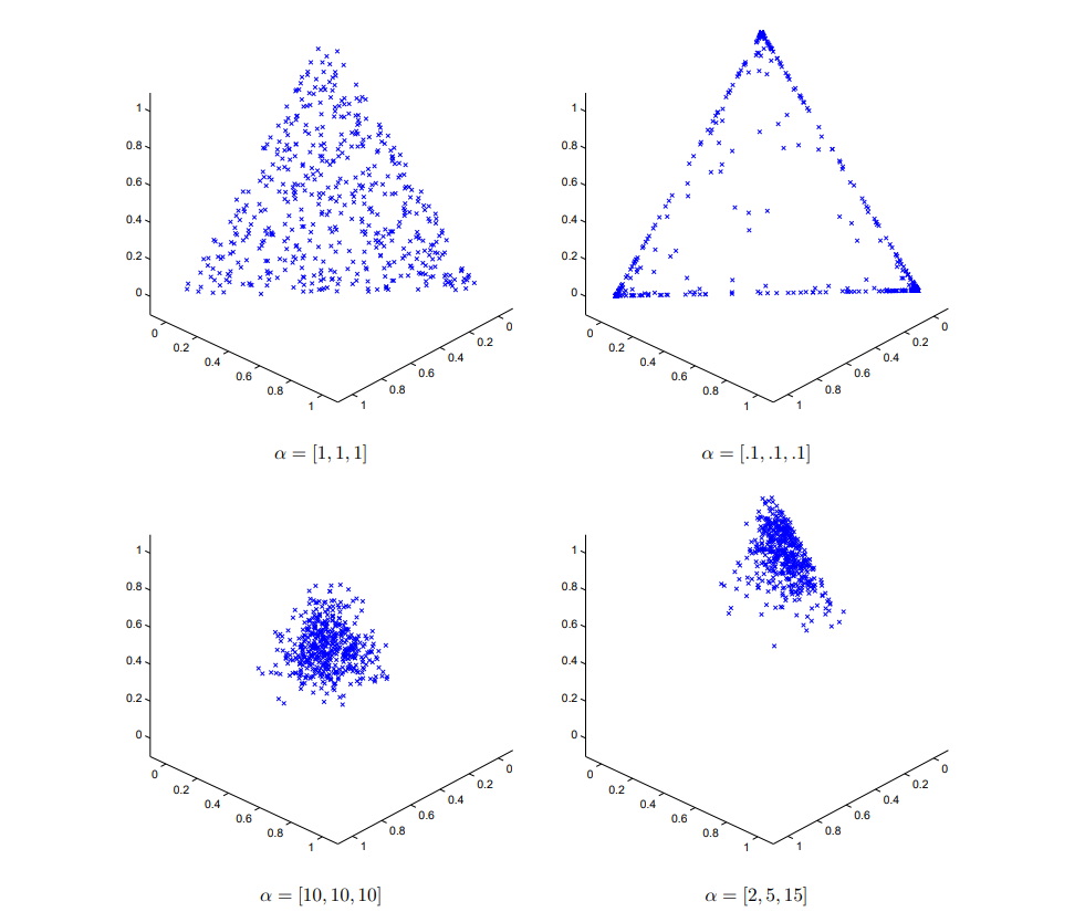
Figure 2.2: Example sampling from a Dirichlet distribution (Frigyik, Kapila and Gupta, 2010)
We also want to talk about the marginal distribution and the conditional distribution of the Dirichlet distribution. These two properties of Dirichlet distribution will play an important role in the stick-breaking process that we will introduce in this chapter:
The marginal distribution is:
\[P(\pi_k) \propto \pi_k^{\alpha_k-1}(1-\pi_k)^{\displaystyle\sum_{i \neq k}\alpha_i -1} = Beta(a_k, \displaystyle\sum_{i \neq k}\alpha_i)\] The conditional distribution of \(\pi_2, \pi_3, ..., \pi_k\) given \(\pi_1\) is:
\[(\pi_2, \pi_3, ..., \pi_K)|\pi_1 \sim (1-\pi_1)Dir(\alpha_2, \alpha_3,..., \alpha_k)\]
2.2 Finite K-component mixture model
After introducing the Dirichlet distribution, we will explain the role that Dirichlet distribution plays in a finite k-component model. Here is an example of a finite K-component Gaussian mixture model.
\[ x_n \stackrel{ind}\sim N(\mu_{z_n}, \sigma)\\ z_n \stackrel{ind}\sim Categorical(\pi_{1:k})\\ \mu_k \stackrel{ind}\sim N(\mu_0, \sigma_0)\\ \pi_{1:k} \sim Dir(\alpha_{1:k})\\ \]
The Dirichlet distribution will give us \(K\) mixture proportions, \(\pi_{1:k}\) that add up to \(1\), where \(\pi_i\) indicates the probability for a data point to fall within the cluster \(i\). The distribution of \(\pi_{1:k}\) is determined by the set of parameters \(\alpha_{1:k}\) of the Dirichlet distribution, which reflects the weights of every mixture from \(\pi_1\) to \(\pi_k\). We also need to determine the parameters associated with each cluster. In the example above, since each cluster follows a normal distribution, the parameter for cluster \(i\) is its mean \(\mu_i\). The set of means, \(\mu_i\)’s, are drawn from a normal distribution with a mean of \(\mu_0\) and standard deviation of \(\sigma_0\). Next, we will draw \(z_n\) from a Categorical distribution \((\pi_{1:k})\) to determine the cluster. Finally, we will draw data point \(x_n\) from a normal distribution with a mean of \(\mu_{z_n}\) and a standard deviation of \(\sigma\).
2.3 Infinite K-component mixture model
However, using a mixture model with only a finite number of components exposes us to selecting an incorrect number of components that do not fit the data, which motivates the use of an infinite-component mixture model. Before we introduce this type of model, we need to first note that the concepts of components and clusters are different. Components are the number of latent groups, but the cluster is the number of components represented in the data. There are \(2\) properties of the number of clusters. First, the number of clusters for \(N\) data is less than or equal to \(K\) and random. Second, it grows with \(N\).
The video below illustrates how the number of clusters grows as we draw more samples from the Dirichlet distribution.
Since the number of clusters will never exceed the value of \(K\), the finite K-component mixture model has limitations. For example, it can not model the groups on social networks because the number of groups will keep growing. The model will not be effective because the max number of clusters is \(K\). The value of finite \(K\) is hard to choose in advance. We do not know about \(K\), and it isn’t easy to infer. To solve this problem, we can choose \(K = \infty\).
2.4 Polya’s Urn
Based on the above the models, a potential question is that how to generate samples from a Dirichlet distribution \(\pi_{1:K} \sim Dir(\alpha_{1:K})\). The Polya’s Urn shown in Figure 2.3 is a common metaphor to help understand sample-drawing process from a Dirichlet distribution. We define \(X_i\) as the \(i_{th}\) sample we draw First, we draw \(X_1 \sim \frac{\alpha}{\parallel \alpha \parallel_1}\), \(\frac{\alpha}{\parallel \alpha \parallel_1}\) is a normalized vector that the sum of all the entries is \(1\). Next, we draw \(X_{n+1} | X_1, \cdots,X_n \sim \frac{\alpha_n}{\parallel \alpha_n \parallel_1}\), where \(\alpha_n = \alpha + \displaystyle\sum_{i = 1}^{n}\delta_{X_i}\). \(\delta_{X_i}\) mean that only the value at \(X_i\) is \(1\) and otherwise the values equals to \(0\). We can repeated this step for infinite number of times. After the process of drawing all the samples, we can calculate the proportion of different clusters \(\pi = (\pi_{1}, \pi_{2}, \pi_{3}, \cdots, \pi_{k})\), where \(\pi_{i}\) is the proportion (weight) of cluster \(k\) through the sampling drawing process.
The following figure shows the process of drawing samples from \(Dir([2,1,1,])\).
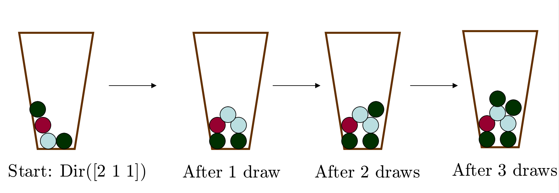
Figure 2.3: Polya urn (Frigyik, Kapila and Gupta, 2010)
Suppose we have \(4\) balls that \(2\) of them are green, \(1\) of them is red, and the other one is light gray. Each color represents a cluster. We randomly draw \(1\) one of these balls, put it back, and add \(1\) ball with the same color into the box. We repeat the process many times, and the proportion of the number of balls in green, red, and light gray will converge to a probability mass function that is a sample in \(Dir([2,1,1])\).
2.5 Stick-breaking process
As shown in Figure 2.5, the stick-breaking process is another metaphor to describe drawing samples from a Dirichlet distribution. The main idea is that break the stick of length \(1\) into \(k\) pieces, and the lengths of \(k\) pieces follow a Dirichlet distribution. Recalling the property of Dirichlet process, we have \(P(\pi_k) \propto \pi_k^{\alpha_k-1}(1-\pi_k)^{\displaystyle\sum_{i \neq k}\alpha_i -1} = Beta(a_k, \displaystyle\sum_{i \neq k}\alpha_i)\) and \((\pi_2, \pi_3, ..., \pi_K)|\pi_1 \sim (1-\pi_1)Dir(\alpha_2, \alpha_3,..., \alpha_k)\):
\[\text{When we are sampling } \pi \sim Dir(\alpha_1, \alpha_2, \alpha_3),\\ V_1 \sim Beta(\alpha_1, \alpha_2 + \alpha_3) \text{, } \pi_1 = V_1\\ V_2 \sim Beta(\alpha_2, \alpha_3)\text{, } \pi_2 = (1-V_1)V_2\\ \pi_3 = 1- \displaystyle\sum_{k = 1}^{2}\pi_k\]
Figure 2.4 is the visualization of the Dirichlet distribution as breaking a stick of length \(1\) into \(3\) pieces. For each value of \(\alpha\), we simulate \(10\) stick-breaking, and each simulation represents a random sample we generate from the Dirichlet distribution.
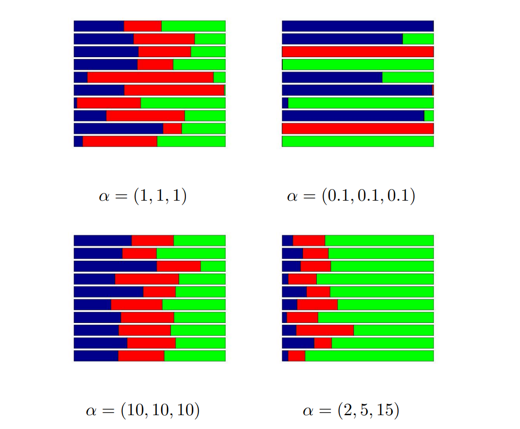
Figure 2.4: Stick breaking examples (Frigyik, Kapila and Gupta, 2010)
We can apply the same idea to find \(K = \infty\) probability that strictly sums to \(1\).
\[V_1 \sim Beta(a_1, b_1) \text{, } \pi_1 = V_1\\ V_2 \sim Beta(a_2, b_2)\text{, } \pi_2 = (1-V_1)V_2\\ V_3 \sim Beta(a_3, b_3)\text{, } \pi_3 = (1-V_1)(1-V_2)V_3\\ \cdots\\ V_k \sim Beta(a_k, b_k)\text{, } \pi_k = [\displaystyle\prod_{j = 1}^{k-1}(1-Vj)] V_k\]
In the Dirichlet process stick-breaking, we define that \(a_k = 1\) and \(b_k = \alpha >0\) to let the sum equals to \(1\), where \(\alpha\) is the concentration parameter of Dirichlet process. In this case, \(V_k\) are independent \(Beta(1, \alpha)\). We called the distribution \((\pi_1, \pi_2, \pi_3, \cdots, \pi_k)\) Griffiths-Engen-McCloskey (GEM) distribution, which is \(\pi = (\pi_1, \pi_2, \pi_3, \cdots, \pi_k) \sim GEM(\alpha)\). The GEM distribution is a Dirichlet process that only takes \(1\) parameter, for instance, we can write \(Dir([1,1,1,1,1])\) as \(GEM(1)\). By limiting the distribution in \(1\) parameter is mainly for simplicity. We will discuss more about Dirichlet Process in Chapter \(3\).
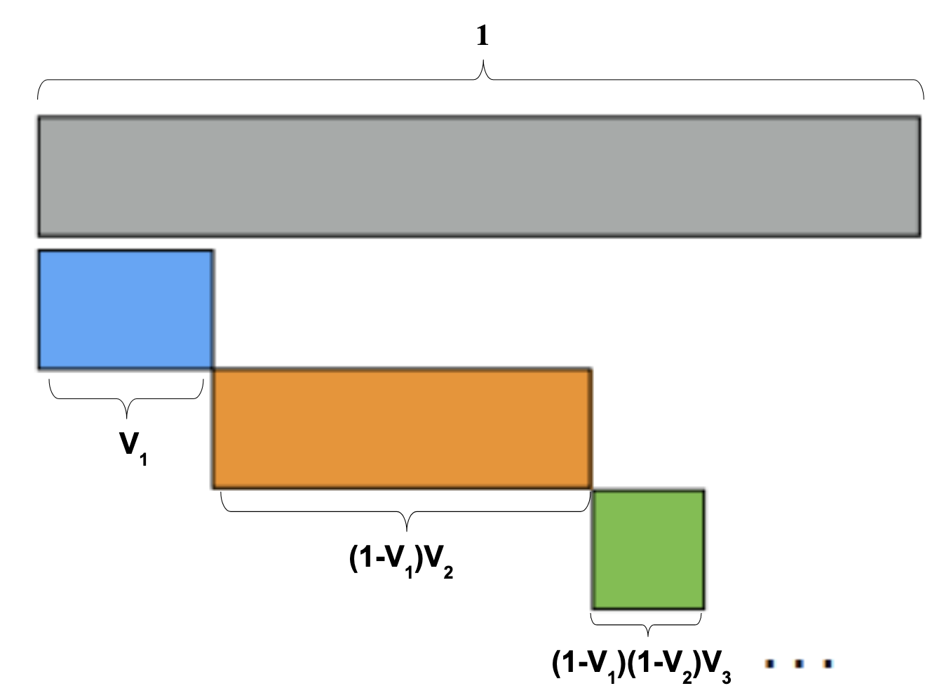
Figure 2.5: Sticking breaking process (Broderick, 2015)
2.6 Appendix
2.6.1 Simulation Codes
The following codes are used to demonstrate how the number of cluster grows with sample size \(N\) in Section 2.5 (Broderick,n.d).
# Illustration of cluster growth
# given a Dirichlet-distributed vector
# with K >> N.
# Copyright (C) 2015, Tamara Broderick
# www.tamarabroderick.com

# useful for sampling from a Dirichlet distribution
library(MCMCpack)

# maximum number of data points to draw
maxN = 1000

# use these parameter by default
K_default = 1000
a_default = 10/K_default
# note: default run with these parameters
# appears at the end

ex4_gen_largeK_count <- function(K,a) {
# Illustrates how number of clusters changes
# with Dirichlet-distributed component probabilities
#
# Args:
#  K: Dirichlet parameter vector length
#  a: Dirichlet parmeter (will be repeated K times)
#
# Returns:
#  Nothing

    # make the Dirichlet draw
    rhomx = rDirichlet(1,rep(a,K))
    # another useful form of rho
    rho = as.vector(rhomx)

    # records which clusters have been sampled so far
    uniq_draws = c()
    # cluster samples in order of appearance (ooa)
    ooa_clust = c()

    for(N in 1:maxN) {
        # draw a cluster assignment from the components
        draw = sample(1:K, size=1, replace=TRUE, prob=rho)
        # update info about cluster draws
        uniq_draws = unique(c(uniq_draws, draw))
        ooa = which(draw == uniq_draws)
        ooa_clust = c(ooa_clust, ooa)

        # plot cluster assignments in order of appearance
        plot(seq(1,N),
            ooa_clust,
            xlab="Sample index",
            ylab="Cluster by order of appearance",
            ylim=c(0,max(10,length(uniq_draws))),
            xlim=c(0,max(10,N)),
            pch=19,
            main=bquote(rho~"~Dirichlet"  # ~"("~.(a)~",...,"~.(a)~")"
                                ~", K="~.(K))
            )

        # Generate a new draw for each press of "enter"
                # Press 'x' when finished
        line <- readline()
        if(line == "x") return("done")
    }
}

# default run with default parameters
ex4_gen_largeK_count(K_default, a_default)
Reference
Broderick, T. (n.d.). Tutorial of Bayesian Nonparametric. Tamara Broderick. Retrieved November 13, 2021, from https://tamarabroderick.com/tutorials.html.
Frigyik, B. A., Kapila, A., & Gupta, M. R. (n.d.). Introduction to the Dirichlet Distribution and Related Process. Retrieved December 3, 2021, from http://mayagupta.org/publications/FrigyikKapilaGuptaIntroToDirichlet.pdf.
Xing, E. P. (n.d.). 19 : Bayesian nonparametrics: Dirichlet processes. Retrieved November 6, 2021, from https://www.cs.cmu.edu/~epxing/Class/10708-14/scribe_notes/scribe_note_lecture19.pdf.