Chapter 4 Dirichlet Process for Survival Analysis

Dirichlet Process mixture models (DPMM) provide flexible data modeling by allowing for countably many mixtures of parametric distributions and have been widely used in different scenarios. In this project, we demonstrate the flexibility and robustness of DPMM by applying it to the setting of survival analysis. Despite the wide use of the Weibull model to fit survival data, its assumption that a finite collection of parameters (i.e., the shape and scale parameters in a Weibull model) could fully describe the data distribution might be naive. There could be a mixing of mechanisms that leads to different event times for different individuals, which motivates mixture models. However, this gives rise to the problem that, in real life, it could be hard to tell the number of components that compose the mixture distribution. To address this issue, in the following sections, we introduce a DP Weibull mixture model developed by Kottas (2006), where both the shape parameter $\alpha$ and $\beta$ are mixed so that a wide range of distribution shapes could be well-modeled.

4.1 Model

Suppose we have a dataset with sample size $n$ , then the Dirichlet process Weibull mixture model can be represented by the following hierarchical model using the notations introduced in Chapter 3:

$t_i\mid a_i,\beta_i \overset{i.i.d}{\sim} Weibull(\alpha_i,\beta_i),\quad i = 1,2,\ldots,n$

$\alpha_i,\beta_i\mid G \overset{i.i.d}{\sim} G,\quad i = 1,2,\ldots,n$

$G\mid v,\gamma,\phi\sim DP(vG_0)$

$v\sim Gamma(v\mid a_v,b_v)$ $G_0(\alpha,\beta\mid \phi,\gamma) = Uniform(\alpha|0,\phi)IGamma(\beta\mid d=2,\gamma)$

$\gamma\sim Gamma(\gamma\mid a_\gamma,b_\gamma)$

$\phi\sim Pareto(\phi\mid a_\phi,b_\phi)$

The parameters for the Weibull kernel, $(\alpha_i,\beta_i)$ , are drawn from the Dirichlet process $G\sim DP(vG_0)$ , where $v$ is the concentration parameter and the base distribution $G_0$ is defined as the product of a uniform distribution and an inverse Gamma distribution. The shape parameter $\alpha$ follows the uniform distribution, while the scale parameter $\beta$ follows the inverse Gamma distribution. In the inverse Gamma distribution, we choose $d=2$ such that $\lambda$ could have a finite variance. That is,

$f(\beta) = \frac{\gamma^d}{\Gamma(d)}x^{-d-1}e^{\frac{-\gamma}{\lambda}}$ and

$E[\beta] = \frac{\gamma}{d-1}=\gamma$ Further, the priors for $\phi$ , $\gamma$ and $v$ are chosen to facilitate Gibbs sampler.

The posterior distribution is then

$F(t;G)=\int Weibull(t\mid\alpha,\beta)G(d\alpha,d\beta)$ where we marginalize over G by integrating out $\alpha$ and $\beta$ .

Choice of $G_0$

Ideally, we would like to select a base distribution $G_0$ to facilitate posterior analysis. Although base distribution $G_0$ that yields a closed form expression for the above formula is not available (Kottas, 2006), setting $G_0(\alpha,\beta\mid \phi,\gamma) = Uniform(\alpha|0,\phi)IGamma(\lambda\mid d=2,\gamma)$ facilitates the numerical integration involved in the computation of the posterior distribution.

However, the choice of $G_0$ is not unique. For example, the R package DPWeibull (Shi, 2020) implements a slightly different choice (Shi et al. 2019). We use the R package DPWeibull for demonstration.

4.2 Simulation

We conducted simulation studies to compare a DP Weibull Mixture model with a traditional Weibull mixture model estimated by the expectation-maximization algorithm in order to demonstrate the flexibility of DPMM. We simulated data using an underlying mixture distribution consisting of three Weibull distributions, and compared the DP Weibull mixture model with a two-component Weibull mixture model that misspecifies the number of components, which is likely to occur in the reality where the correct number of components is unknown. Specifically, the three Weibull distributions contributing to the underlying truth are $Weibull(2,2)$ , $Weibull(1.5,3)$ , and $Weibull(3,3.2)$ , and each contributes equally with a weight of $1/3$ ¹.

Figure 4.1 shows the survival distribution and hazard function of the mixture distribution we use for simulation. The hazard function shown in Figure 4.1, $h(t) = \frac{f(t)}{S(t)}$ , is often used to characterize a survival distribution. Conceptually, the hazard function describes the conditional probability for the failure event (i.e., death in this case) to occur at time $t$ given that the patient has survived up to time $t$ . For our simulated data, the hazard first increases up to $t=4$ when it starts to decrease. However, it is well-known that the hazard function of Weibull distribution is monotone. Thus, although the simulated data is generated from a mixture of Weibull models, any single Weibull model would fail to fit the data adequately.

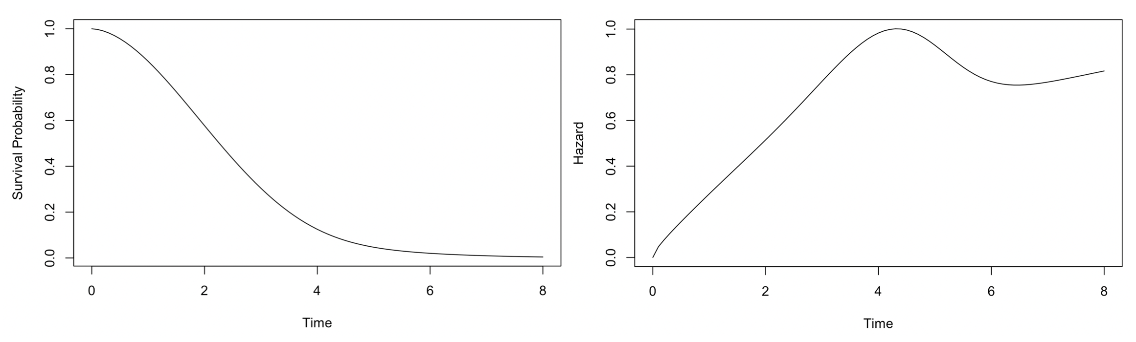
Figure 4.1: The survival distribution and hazard function of a mixture of three Weibull distributions used for simuation

We further chose three levels of random censoring, 10%, 20%, and 30%, to compare the performances of the two models under different censoring rates. Figure 4.2 summarizes the performance of the Dirichlet process (DP) Weibull mixture model and a Weibull mixture model with two components under the three levels of censoring rates. As the DP Weibull mixture model is free from misspecification of the number of components, it has smaller mean squared errors (MSEs) than a Weibull mixture model with two components. As the censoring rates increases, the proportion of exact observation decreases. For example, a 30% censoring means that, for 30% of observed data, we only know their survival time is longer than their censoring time. Thus, as censoring rates increase, we expect the mean squared errors to increase for both models, as confirmed by Figure 4.2.

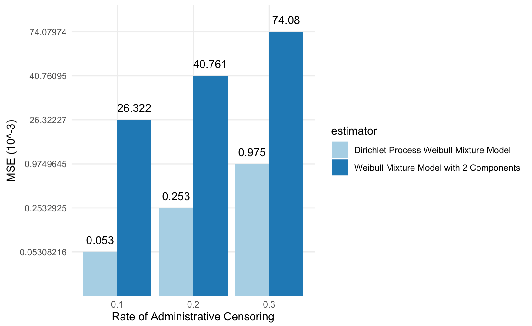
Figure 4.2: MSE (in 10^-3) of the DP Weibull Mixture models and the two-component Weibull Mixture models under 10% ,20%, and 30% random censoring

Figures 4.3-4.5 show the estimated survival distribution and the 95% confidence interval (CI) of the two models. The estimates the DP mixture model produces are much closer to the underlying truth than a misspecified mixture model, especially when the censoring rate is high. That being said, we note that both models appear to overestimate the survival probability. We also note that at a high censoring rate, i.e., 30% random censoring, the 95% confidence interval of the DP mixture model barely captures the underlying truth, while the 95% confidence interval of the mixture model manages to do a slightly better job due to its wide width. Nonetheless, the DP Weibull mixture model can still produce a more accurate estimation than a conventional mixture model.

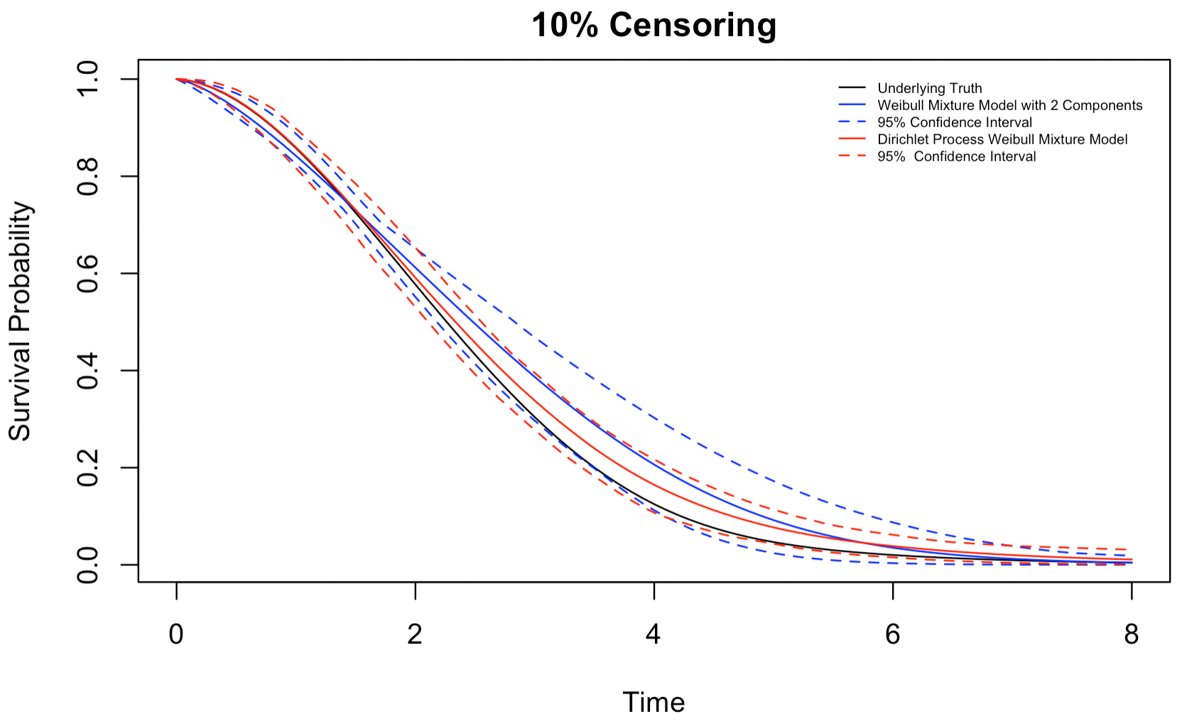
Figure 4.3: Estimates for a mixture of 3 Weibull distributions,10% censoring

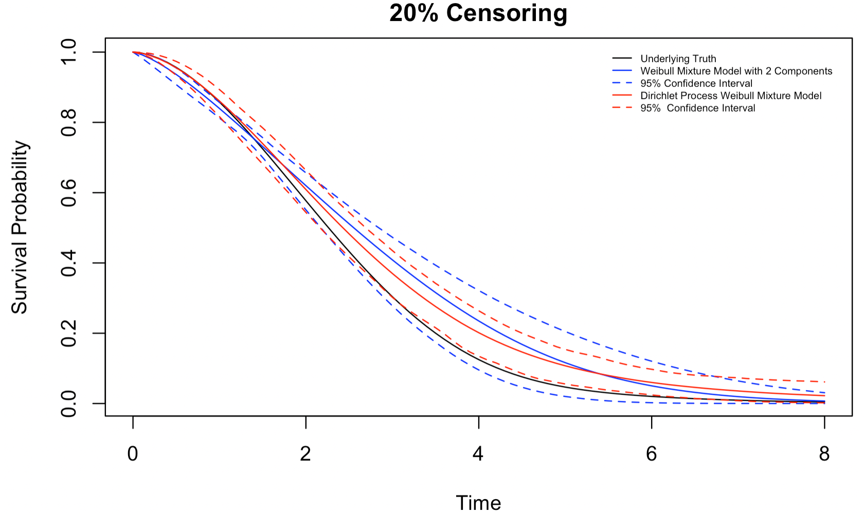
Figure 4.4: Estimates for a mixture of 3 Weibull distributions,20% censoring

Figure 4.5: Estimates for a mixture of 3 Weibull distributions,30% censoring

4.3 Case Study

To demonstrate the use of the Dirichlet process Weibull mixture model, we consider a dataset by Haupt and Mansmann (1995) of the survival time in months for patients with liver metastases, which is readily available in the R package locfit. This dataset is also used by Kottas (2006) for demonstration. Figure 4.6 shows the smoothed hazard function $h(t)$ given by the kernel-based methods provided by the R package muhaz. The hazard increases until around 20 months, and flattens during 20-35 months, while it appears to start to decrease after 35 months. Similar to our simulation setting, the non-monotone hazard indicates that fitting a single Weibull model would fail to characterize the data.

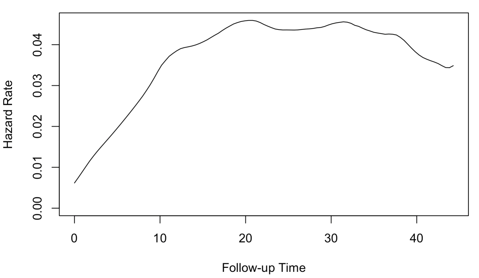
Figure 4.6: Smoothed kernel-based hazard function for liver metastases survival time

Figure 4.7 shows the estimated survival distribution and hazard of the liver metastases dataset along with their 95% posterior confidence interval (2006). We note that the difference in the choice of base distribution $G_0$ by Kottas (2006) and the R package DPWeibull leads to different quantitative hazard estimates. However, both demonstrated trends in the original study by Haupt and Mansmann (1995). The estimated hazard increases until roughly 15 months, which levels off and starts to decline after 35 months, which, as Kottas (2006) noted, might be attributed to the fact that roughly 96%² of exact observations occurred before the 35th month.

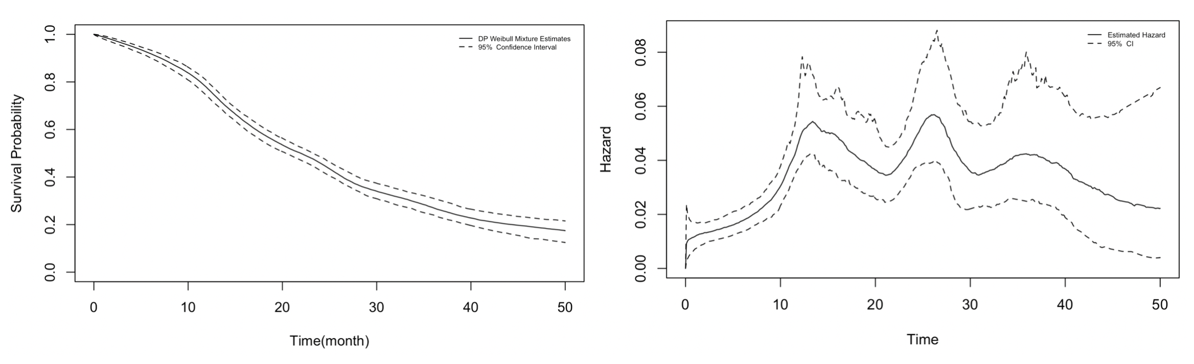
Figure 4.7: Estimated survival distribution and hazard of liver metastases based on the DP Weibull mixture model

4.4 Appendix

4.4.1 Simulation Codes

#### Load Libraries 

library(survival)
library(DPWeibull)
library(Rsolnp)


### Function to Generate Data from a Mixture of 3 Weibull Components

full.weib.mixed.simulate = function(n, coeff, weibpar1,weibpar2,weibpar3,cpar) {    
  count1=0;count2=0;count3=0
  j = 0
  output = NULL
  while (j < n) {                                   # iterate until a sample of size n is obtained
    mod.sel = which(rmultinom(1,1,coeff)==1)
    if (mod.sel == 1){
      count1=count1+1
      t = rweibull(1, shape=weibpar1[1], scale=weibpar1[2])             
    }
    else if (mod.sel == 2) {
      count2=count2+1
      t = rweibull(1, shape=weibpar2[1], scale=weibpar2[2])     
    }
    else{ #mod.sel == 2
      count3=count3+1
      t = rweibull(1, shape=weibpar3[1], scale=weibpar3[2]) 
    }
     cens.t = rexp(1,cpar)                  # generate a forward censoring time (this form of ltr + cens, ensures the censoring time is included in the cohort)
    surv.time = ifelse(t <= cens.t, t, cens.t)  # take the minimum to
    delta = ifelse(t <= cens.t, 1, 0)           # generate status indicator
    output = rbind(output, c(t, delta)) 
  
    j=j+1
  }
  output = data.frame(output)
  
  dimnames(output)[[2]] = c("time","indicator") # give names to output columns for easy access

  return(output)
}





# load libraries

library(survival)
library(DPWeibull)
library(Rsolnp)

### Likelihoods Function for Two-Component Weibull Mixture 

full.mixture.likelihood.2Weib<-function(param,fwrd.dat){
  
  weib1.coef= param[1];weib2.coef= param[2];weib1.shp= param[3];weib1.scl= param[4];weib2.shp= param[5];weib2.scl= param[6]
  #print(c(weib1.coef,weib2.coef,weib1.shp, weib1.scl, weib2.shp,weib2.scl))
  f<-function(x,weib1.coef,weib2.coef,weib1.shp, weib1.scl, weib2.shp,weib2.scl){
    return(weib1.coef*dweibull(x,shape=weib1.shp,scale = weib1.scl)+weib2.coef*dweibull(x,shape=weib2.shp,scale = weib2.scl))
  }
  
  S<-function(x,weib1.coef,weib2.coef,weib1.shp, weib1.scl, weib2.shp,weib2.scl){
    return(weib1.coef*(1-pweibull(x,shape=weib1.shp,scale = weib1.scl))+weib2.coef*(1-pweibull(x,shape=weib2.shp,scale = weib2.scl)))
  }

  fail.vals = log1p(f(fwrd.dat$time,weib1.coef=weib1.coef,weib2.coef=weib2.coef,weib1.shp=weib1.shp, weib1.scl=weib1.scl, weib2.shp=weib2.shp,weib2.scl=weib2.scl)-1)*fwrd.dat$indicator
  
  cens.vals = log1p(S(fwrd.dat$time,weib1.coef=weib1.coef,weib2.coef=weib2.coef,weib1.shp=weib1.shp, weib1.scl=weib1.scl, weib2.shp=weib2.shp,weib2.scl=weib2.scl)-1)*(1-fwrd.dat$indicator)

  
  like.result = -sum(fail.vals)-sum(cens.vals)

  like.result=exp(like.result)
  #print(c(sum(fail.vals),sum(cens.vals)))
  return(like.result)
}

### Data Generation 

# parameters for simulation

coeff=rep(1/3,3)
MSE.times = seq(0,8,by=0.1) 
weibpar1=c(2,2);weibpar2=c(1.5,3);weibpar3=c(3,3.2)
# 30% censoring:cpar = 0.15
# 20% censoring:cpar = 0.09
# 10% censoring:cpar = 0.045
cpar = 0.09 

msim=50
nsim=200

set.seed(2021)
full.weib.mixed.sim.data=list()
for(i in 1:msim){
  full.weib.mixed.sim.data[[i]] =full.weib.mixed.simulate(nsim,coeff =coeff,weibpar1 = weibpar1,weibpar2 = weibpar2,weibpar3=weibpar3,cpar=0.09)
}
sum(full.weib.mixed.sim.data[[1]]$indicator==1)/nsim




### two-component Weibull Mixture Estimates 

eqn1=function(x,fwrd.dat){
    return(x[1]+x[2]-1)
}

weib1.coef=0.5;weib2.coef=0.5;weib1.shp=1.8; weib1.scl=1.8; weib2.shp=3;weib2.scl=3
x0=c(weib1.coef,weib2.coef,weib1.shp, weib1.scl, weib2.shp,weib2.scl)

opt.mixture.2Weib = list()
for(i in 1:msim){
  opt.mixture.2Weib[[i]]=solnp(c(weib1.coef,weib2.coef,weib1.shp, weib1.scl, weib2.shp,weib2.scl), fun=full.mixture.likelihood.2Weib,fwrd.dat=full.weib.mixed.sim.data[[i]], eqfun = eqn1,eqB = 0,control=list(trace=0), LB=c(0,0,0,0,0,0), UB=c(1,1,Inf,Inf,Inf,Inf))$pars
}

res = matrix(unlist(opt.mixture.2Weib),nrow =50,byrow = T)
res


## plot


plot(MSE.times, 1-(coeff[1]*pweibull(MSE.times, weibpar1[1],weibpar1[2])+coeff[2]*pweibull(MSE.times, weibpar2[1],weibpar2[2])+coeff[3]*pweibull(MSE.times, weibpar3[1],weibpar3[2])),type='l')
for (i in 1:msim) {
  
  lines(MSE.times,opt.mixture.2Weib[[i]][1]*(1 - pweibull(MSE.times, shape=opt.mixture.2Weib[[i]][3], scale=opt.mixture.2Weib[[i]][4]))+opt.mixture.2Weib[[i]][2]*(1 - pweibull(MSE.times, shape = opt.mixture.2Weib[[i]][5], scale=opt.mixture.2Weib[[i]][6])),col='red')
  
}



### DP Weibull Mixture Estimates 

DP.lst=list() # no covariate
for(i in 1:msim){
  DP.lst[[i]]=dpweib(Surv(time,indicator)~1,data=full.weib.mixed.sim.data[[i]],predtime=MSE.times)
}



### MSE and 95% CI 

mixture.2weib.MSE = rep(0, msim);DPM.MSE = rep(0, msim)
# a matrix to record the estimates by conventional mixture model for each simulated dataset
mixture.2weib.est.matrix = matrix(NA,msim,length(MSE.times)) 
# a matrix to record the estimates by DPM for each simulated dataset
DPM.est.matrix= matrix(NA,msim,length(MSE.times)) 

# underlying truth
truth = 1-(coeff[1]*pweibull(MSE.times, weibpar1[1],weibpar1[2])+coeff[2]*pweibull(MSE.times, weibpar2[1],weibpar2[2])+coeff[3]*pweibull(MSE.times, weibpar3[1],weibpar3[2]))
  
for (i in 1:msim) {

   mixture.2weib.est=opt.mixture.2Weib[[i]][1]*(1 - pweibull(MSE.times, shape=opt.mixture.2Weib[[i]][3], scale=opt.mixture.2Weib[[i]][4]))+opt.mixture.2Weib[[i]][2]*(1 - pweibull(MSE.times, shape = opt.mixture.2Weib[[i]][5], scale=opt.mixture.2Weib[[i]][6]))
  mixture.2weib.est.matrix[i,]=mixture.2weib.est
  
  mixture.2weib.MSE[[i]] = sum((MSE.times[2] - MSE.times[1])*( mixture.2weib.est-truth)^2)
  
  DPM.est = DP.lst[[i]]$Spred
  DPM.est.matrix[i,]=DPM.est
  DPM.MSE[[i]] = sum((MSE.times[2] - MSE.times[1])*( DPM.est -truth)^2)
}

# MSE
mean(mixture.2weib.MSE); var(DPM.MSE)

# empirical 95% confidence intervals
mixture.2weib.est.mean=apply(mixture.2weib.est.matrix,2,mean)
DPM.est.mean=apply(DPM.est.matrix,2,mean)
mixture.2weib.est.low=apply(mixture.2weib.est.matrix,2,function(x){
  quantile(x,0.025)
})
mixture.2weib.est.high=apply(mixture.2weib.est.matrix,2,function(x){
  quantile(x,0.975)
})
DPM.est.low=apply(DPM.est.matrix,2,function(x){
  quantile(x,0.025)
})
DPM.est.high=apply(DPM.est.matrix,2,function(x){
  quantile(x,0.975)
})

# Plot
plot(MSE.times,truth,type='l',xlab='Time',ylab='Survival Probability',main="10% Censoring")
lines(MSE.times,mixture.2weib.est.mean,type='l',col='blue');lines(MSE.times,mixture.2weib.est.low, lty=2,col='blue');lines(MSE.times,mixture.2weib.est.high, lty=2,col='blue')
legend('topright',inset=0.02,legend=c("Underlying Truth", "Weibull Mixture Model with 2 Components","95% Confidence Interval"),
       col=c("black", "blue","blue"), lty=c(1,1,2), cex=0.5,box.lty=0)

plot(MSE.times,truth,type='l',xlab='Time',ylab='Survival Probability',main="10% Censoring")
lines(MSE.times,DPM.est.mean,type='l',col='red');lines(MSE.times,DPM.est.low, lty=2,col='red');lines(MSE.times,DPM.est.high, lty=2,col='red')
legend('topright',inset=0.02, legend=c("Underlying Truth", "Dirichlet Process Weibull Mixture Model","95%  Confidence Interval"),
       col=c("black", "red","red"), lty=c(1,1,2), cex=0.5,box.lty=0)

4.4.2 Liver Metastases Dataset

library(dplyr)
library(locfit)
data(livmet)
# exact observation distribution
sum((livmet%>%filter(z==1))$t<35)/nrow(livmet%>%filter(z==1))
# fit model
DP.livmet=dpweib(Surv(t,z)~1,data=livmet,predtime=seq(0,50,by=0.1),a=3,b=0.05)
# plot
plot(seq(0,50,by=0.1),DP.livmet$Spredu,lty=2,type='l',xlab='Time(month)',ylab='Survival Probability',ylim=c(0,1))
lines(seq(0,50,by=0.1),DP.livmet$Spred,lty=1,type='l')
lines(seq(0,50,by=0.1),DP.livmet$Spredl,lty=2,type='l')
legend('topright',inset=0.02, legend=c("DP Weibull Mixture Estimates","95%  Confidence Interval"), lty=c(1,2), cex=0.5,box.lty=0)
plot(seq(0,50,by=0.1),DP.livmet$hpredu,lty=2,type='l',xlab = 'Time', ylab='Hazard')
lines(seq(0,50,by=0.1),DP.livmet$hpredl,lty=2)
lines(seq(0,50,by=0.1),DP.livmet$hpred,lty=1)
legend('topright',inset=0.02, legend=c("Estimated Hazard","95%  CI"), lty=c(1,2), cex=0.5,box.lty=0)

Reference

Haupt, G. and Mansmann, U. (1995). CART for Survival Data. Statlib Archive, http://ftp.uni-bayreuth.de/math/statlib/S/survcart

Kottas, A. (2006). Nonparametric Bayesian survival analysis using mixtures of Weibull distributions. Journal of Statistical Planning and Inference, 136(3), 578-596. doi:10.1016/j.jspi.2004.08.009

Shi, Y., Martens, M., Banerjee, A., & Laud, P. (2019). Low Information Omnibus (LIO) Priors for Dirichlet Process Mixture Models. Bayesian Analysis, 14(3). doi:10.1214/18-ba1119

Shi, Y. (2020). DPWeibull: Dirichlet Process Weibull Mixture Model for Survival Data . R package version 1.18 (unpublished)

See Appendix for more details↩︎
See Appendix for more details↩︎